從零開始學AI圖型辨識(基礎篇)

2023/01/01閱讀時間約 40 分鐘

matplotlib

pip install matplotlib

Matplotlib 建新圖，基本步驟

Step 1 ：Prepare Data
Step 2 ：Create Plot
Step 3 ：Plot
Step 4 ：Customize Plot
Step 5 ：Save Plot
Step 6 ：Show Plot

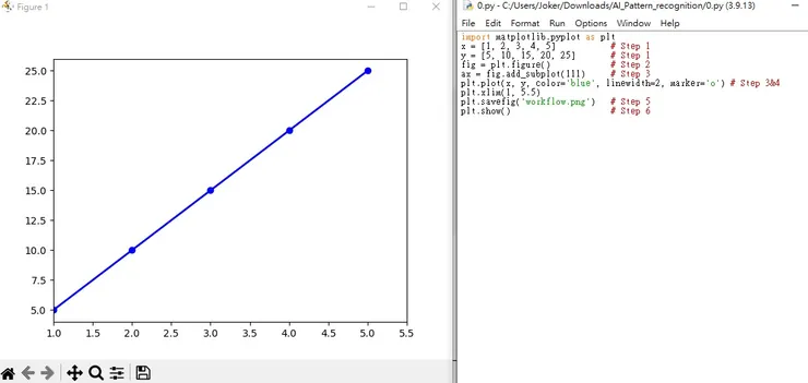
import matplotlib.pyplot as plt
x = [1, 2, 3, 4, 5]           # Step 1 載入數據資料
y = [5, 10, 15, 20, 25]       # Step 1 載入數據資料
fig = plt.figure()            # Step 2 載入plot函式
ax = fig.add_subplot(111)     # Step 3 建立圖表
plt.plot(x, y, color='blue', linewidth=2, marker='o') # Step 3&4 將資料放入plt內並設定相關參數
plt.xlim(1, 5.5)              #設定 x 軸        
plt.savefig('workflow.png')   # Step 5 輸出圖檔
plt.show()                    # Step 6 顯示於畫面上

figure() ，用於建一個新的圖表視窗。

add_subplot() 是一個方法，用於向圖表視窗中添加子圖。

111 是一個三位數的常數，用於指定子圖的布局。
第一位數字 1 表示圖表視窗被分成了一行
第二位數字 1 表示圖表視窗被分成了一列
第三位數字 1 表示第一個子圖
因此，這個程式會在圖表視窗中增加一個填滿整個視窗的子圖

設定X 軸範圍限制，可以使用 xlim() 和 set_xlim() 方法。
設定Y 軸範圍限制，可以使用 ylim() 和 set_ylim() 方法。

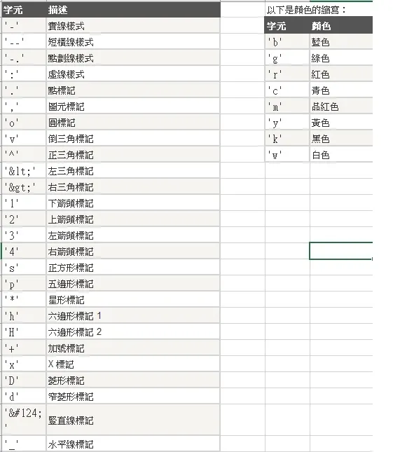
基礎 plot

顏色設定

plt.plot(years,pops,color=(255/255,100/255,100/255))

設定label

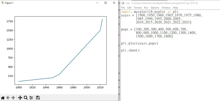
import matplotlib.pyplot as plt
years = [1900,1950,1960,1965,1970,1975,1980,
        1985,1990,1995,2000,2005,
        2010,2015,2020,2021,2022,2023]
pops = [100,200,300,400,500,600,700,
        800,900,1000,1100,1200,1300,1400,
        1500,1600,1700,1800]
#plt.plot(years,pops)
plt.plot(years,pops,color=(255/255,100/255,100/255))
plt.title("Test Image") # title
plt.ylabel("billions") # y label
plt.xlabel("year") # x label
plt.show()

使用中文

https://source.typekit.com/source-han-serif/tw/

下載

將下載的字體與程式放在同目錄下

import numpy as np 
from matplotlib import pyplot as plt 
import matplotlib
years = [1900,1950,1960,1965,1970,1975,1980,
        1985,1990,1995,2000,2005,
        2010,2015,2020,2021,2022,2023]
pops = [100,200,300,400,500,600,700,
        800,900,1000,1100,1200,1300,1400,
        1500,1600,1700,1800]
#plt.plot(years,pops)
plt.plot(years,pops,color=(255/255,100/255,100/255))
fontx = matplotlib.font_manager.FontProperties(fname="SourceHanSerifTC-Bold.otf")
plt.title("測試圖", fontproperties=fontx) # title
plt.ylabel("這是Y軸", fontproperties=fontx) # y label
plt.xlabel("這是X軸", fontproperties=fontx) # x label
plt.show()

使用系統預設中文

import numpy as np 
from matplotlib import pyplot as plt 
import matplotlib
years = [1900,1950,1960,1965,1970,1975,1980,
        1985,1990,1995,2000,2005,
        2010,2015,2020,2021,2022,2023]
pops = [100,200,300,400,500,600,700,
        800,900,1000,1100,1200,1300,1400,
        1500,1600,1700,1800]
#plt.plot(years,pops)
plt.plot(years,pops,color=(255/255,100/255,100/255))
fontx = matplotlib.font_manager.FontProperties(fname="SourceHanSerifTC-Bold.otf")
plt.title("測試圖", fontproperties=fontx) # title
plt.ylabel("這是Y軸", fontproperties=fontx) # y label
plt.xlabel("這是X軸", fontproperties=fontx) # x label
plt.show()
a=sorted([f.name for f in matplotlib.font_manager.fontManager.ttflist])
for i in a:
    print(i)
plt.plot(years,pops,color=(255/255,100/255,100/255))    
plt.rcParams['font.sans-serif']=['Microsoft JhengHei']
plt.rcParams['axes.unicode_minus'] = False
plt.title("測試圖") # title
plt.ylabel("這是Y軸") # y label
plt.xlabel("這是X軸") # x label
plt.show()

增加第二條線

import numpy as np 
from matplotlib import pyplot as plt 
import matplotlib
years = [1900,1950,1960,1965,1970,1975,1980,
        1985,1990,1995,2000,2005,
        2010,2015,2020,2021,2022,2023]
pops = [100,200,300,400,500,600,700,
        800,900,1000,1100,1200,1300,1400,
        1500,1600,1700,1800]
nlines = [1,2,3,4,5,6,7,8,9,10,11,12,13,14,15,16,17,18]
#plt.plot(years,pops)
plt.plot(years,pops,color=(255/255,100/255,100/255))
plt.plot(years,nlines, '--', color=(100/255,100/255,255/255))
fontx = matplotlib.font_manager.FontProperties(fname="SourceHanSerifTC-Bold.otf")
plt.title("測試圖", fontproperties=fontx) # title
plt.ylabel("這是Y軸", fontproperties=fontx) # y label
plt.xlabel("這是X軸", fontproperties=fontx) # x label
plt.show()

import numpy as np 
from matplotlib import pyplot as plt 
import matplotlib
years = [1900,1950,1960,1965,1970,1975,1980,
        1985,1990,1995,2000,2005,
        2010,2015,2020,2021,2022,2023]
pops = [100,200,300,400,500,600,700,
        800,900,1000,1100,1200,1300,1400,
        1500,1600,1700,1800]
nlines = [1,2,3,4,5,6,7,8,9,10,11,12,13,14,15,16,17,18]
#plt.plot(years,pops)
plt.plot(years,pops,color=(255/255,100/255,100/255))
plt.plot(years,nlines, '^', color='c')
fontx = matplotlib.font_manager.FontProperties(fname="SourceHanSerifTC-Bold.otf")
plt.title("測試圖", fontproperties=fontx) # title
plt.ylabel("這是Y軸", fontproperties=fontx) # y label
plt.xlabel("這是X軸", fontproperties=fontx) # x label
plt.show()

相關設定變化

import numpy as np 
from matplotlib import pyplot as plt 
import matplotlib
years = [1900,1950,1960,1965,1970,1975,1980,
        1985,1990,1995,2000,2005,
        2010,2015,2020,2021,2022,2023]
pops = [100,200,300,400,500,600,700,
        800,900,1000,1100,1200,1300,1400,
        1500,1600,1700,1800]
nlines = [1,2,3,4,5,6,7,8,9,10,11,12,13,14,15,16,17,18]
lines = plt.plot(years,pops,years,nlines)
# 設定第一條折線的顏色為藍色
lines[0].set_color('blue')
# 設定第二條折線的顏色為紅色
lines[1].set_color('r')
# 設定第一條折線的數據標記的形狀為圓形
lines[0].set_marker('o')
# 設定第二條折線的數據標記的形狀為三角形
lines[1].set_marker('^')
#plt.plot(years,pops)
#plt.plot(years,pops,color=(255/255,100/255,100/255))
#plt.plot(years,nlines, '^', color='c')
fontx = matplotlib.font_manager.FontProperties(fname="SourceHanSerifTC-Bold.otf")
plt.title("測試圖", fontproperties=fontx) # title
plt.ylabel("這是Y軸", fontproperties=fontx) # y label
plt.xlabel("這是X軸", fontproperties=fontx) # x label
plt.show()

plt.grid()

plt.grid(True)

linewidth

import numpy as np 
from matplotlib import pyplot as plt 
import matplotlib
years = [1900,1950,1960,1965,1970,1975,1980,
        1985,1990,1995,2000,2005,
        2010,2015,2020,2021,2022,2023]
pops = [100,200,300,400,500,600,700,
        800,900,1000,1100,1200,1300,1400,
        1500,1600,1700,1800]
nlines = [1,2,3,4,5,6,7,8,9,10,11,12,13,14,15,16,17,18]
lines = plt.plot(years,pops,years,nlines)
# 設定第一條折線的顏色為藍色
lines[0].set_color('blue')
# 設定第二條折線的顏色為紅色
lines[1].set_color('r')
# 設定第一條折線的數據標記的形狀為圓形
lines[0].set_marker('o')
# 設定第二條折線的數據標記的形狀為三角形
lines[1].set_marker('^')
plt.grid(True)
# 設定第一條折線的線寬為 2 像素
lines[0].set_linewidth(2)
# 設定第二條折線的線寬為 4 像素
lines[1].set_linewidth(4)
#plt.plot(years,pops)
#plt.plot(years,pops,color=(255/255,100/255,100/255))
#plt.plot(years,nlines, '^', color='c')
fontx = matplotlib.font_manager.FontProperties(fname="SourceHanSerifTC-Bold.otf")
plt.title("測試圖", fontproperties=fontx) # title
plt.ylabel("這是Y軸", fontproperties=fontx) # y label
plt.xlabel("這是X軸", fontproperties=fontx) # x label
plt.show()

結合Numpy

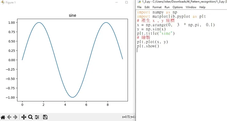
import numpy as np 
import matplotlib.pyplot as plt 
# 產生 x , y 座標
# 生成 0 到 3π 的數值範圍，並且每次递增 0.1
x = np.arange(0,  3  * np.pi,  0.1) 
y = np.sin(x)
plt.title("sine")  
# 繪製
plt.plot(x, y) 
plt.show()

arange() 函數，用於生成數值範圍的數組。

import numpy as np
# 生成 0 到 10 的數值範圍，並且每次递增 1
x = np.arange(0, 11)
print(x)

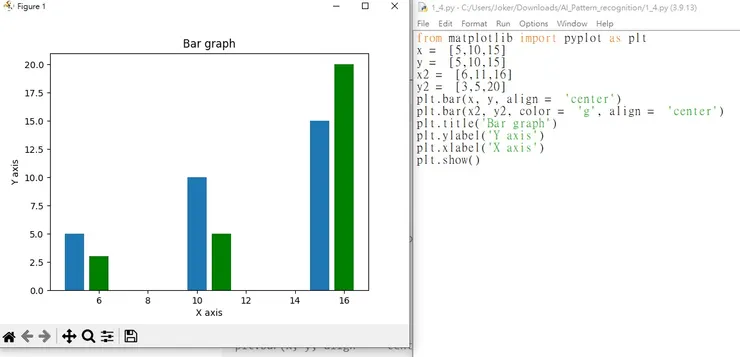
bar()

from matplotlib import pyplot as plt 
x =  [5,10,15] 
y =  [5,10,15] 
x2 =  [6,11,16] 
y2 =  [3,5,20] 
plt.bar(x, y, align =  'center') 
plt.bar(x2, y2, color =  'g', align =  'center') 
plt.title('Bar graph') 
plt.ylabel('Y axis') 
plt.xlabel('X axis') 
plt.show()

subplot()

subplot(nrows, ncols, nsubplot)

nrows：列數
ncols：行數
nsubplot：第n個子圖
如果nrows, ncols, nsubplot數字都在0~9之間的話，可以簡寫成如subplot(321)，表示為將子圖分成3列2行(共6個子圖)中的第1個。

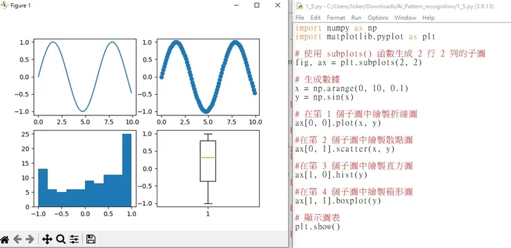
import numpy as np
import matplotlib.pyplot as plt
# 使用 subplots() 函數生成 2 行 2 列的子圖
fig, ax = plt.subplots(2, 2)
# 生成數據
x = np.arange(0, 10, 0.1)
y = np.sin(x)
# 在第 1 個子圖中繪製折線圖
ax[0, 0].plot(x, y)
#在第 2 個子圖中繪製散點圖
ax[0, 1].scatter(x, y)
#在第 3 個子圖中繪製直方圖
ax[1, 0].hist(y)
#在第 4 個子圖中繪製箱形圖
ax[1, 1].boxplot(y)
# 顯示圖表
plt.show()

legend 圖標

plt.legend(labels, loc=’位置’)

loc 參數指定圖例的位置: upper left、lower right。

import matplotlib.pyplot as plt
Taipei_temp = [10.1, 12.2, 13.3, 14.5, 16.6, 17.7, 18.8, 19.9, 20, 21.9]
Taichung_temp = [23.5, 23.8, 23.7, 23.5, 23.6, 23.6, 23.8, 24.3, 24.2, 24.2]
Kaohsiung_temp = [25.1, 25.4, 25.4, 24.9, 25.4, 25.5, 25.6, 26.1, 25.9, 26.3]
year = range(2013, 2023)
plt.plot(year, Taipei_temp, color = 'blue', marker='o', linestyle = '--', label='Taipei')
plt.plot(year, Taichung_temp, color = 'orange', marker='o', linestyle = '-', label='Taichung')
plt.plot(year, Kaohsiung_temp, color = 'green', marker='.', linestyle = '-.', label='Kaohsiung')
plt.legend(loc = 'upper left')
plt.xlabel('Year', color = 'red')
plt.ylabel('Temperature', color = 'red')
plt.title('10-year Average Temperature', color = 'red')
plt.show()

OPEN-CV

關於 open cv 的基礎使用，可參照

圖形辨識筆記-OPEN CV 此文章

當瞭解了基本的 open cv 使用方式後，

我們完成了圖形辨識~尋寶遊戲

的練習後

即可參考 OpenCV 圖轉動漫

此篇文章，了解邊框線取得等方式

進而在學習圖轉文此篇

了解 OCR，光學字元辨識(Optical Character Recognition)

此時，我們知道了躁點的事，也學習到方便的 Pillow 圖像處理的 Python 庫

簡易open cv美肌

透過cv2.bilateralFilter ， OpenCV 中這函數，用於對圖像進行雙邊濾波處理。

它的參數如下：

src：要進行濾波的圖像，一般為灰度圖或彩色圖。
d：濾波器直徑，它決定了濾波半徑。一般來說，較大的直徑會使濾波更加平滑，但同時也會降低邊緣保留能力。
sigmaColor：顏色空間的標準差，決定了濾波器對顏色的敏感程度。較大的標準差會使濾波更加平滑，但同時也會降低邊緣保留能力。
sigmaSpace：坐標空間的標準差，決定了濾波器對像素位置的敏感程度。較大的標準差會使濾波更加平滑，但同時也會降低邊緣保留能力。

通過調整這些參數，你可以控制濾波器的性能，例如平滑程度和邊緣保留能力。

import cv2
source = cv2.imread("test2.jpg")
target = cv2.bilateralFilter(src=source, d=0, sigmaColor=30, sigmaSpace=15)
cv2.imshow("source", source)
cv2.imshow("target", target)
cv2.waitKey()
cv2.destroyAllWindows()

Pillow 圖像處理

pip install pillow

其簡單的操作如:

from PIL import Image
# 讀取圖片
im = Image.open('image.jpg')
# 縮小圖片
im = im.resize((100, 100))
# 旋轉圖片
im = im.rotate(45)
# 翻轉圖片
im = im.transpose(Image.FLIP_LEFT_RIGHT)
# 保存圖片
im.save('modified.jpg')

PyQt5

安裝 PyQt5

pip install pyqt5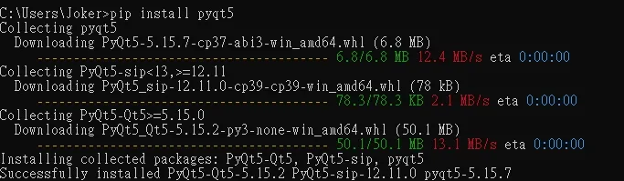

import sys
from PyQt5.QtWidgets import QApplication, QWidget
# 創建應用程式和視窗
app = QApplication(sys.argv)
window = QWidget()
window.setWindowTitle('My Window')
window.show()
# 進入應用程式的主循環
sys.exit(app.exec_())

安裝 cmake

https://cmake.org/download/

dlib

pip install dlib
or
python setup.py install

imutils

pip install imutils

範例:

# pip install imutils
import dlib
import cv2
import imutils
# 讀取照片圖檔
img = cv2.imread('test.jpg')
# 縮小圖片
img = imutils.resize(img, width=640)
# Dlib 的人臉偵測器
detector = dlib.get_frontal_face_detector()
# 偵測人臉
face_rects = detector(img, 0)
# 取出所有偵測的結果
for i, d in enumerate(face_rects):
  x1 = d.left()
  y1 = d.top()
  x2 = d.right()
  y2 = d.bottom()
  # 以方框標示偵測的人臉
  cv2.rectangle(img, (x1, y1), (x2, y2), (0, 255, 0), 4, cv2.LINE_AA)
# 顯示結果
cv2.imshow("Face Detection", img)
cv2.waitKey(0)
cv2.destroyAllWindows()

下載 dlib 預設模型 dlib模型

import cv2
import dlib
detector = dlib.get_frontal_face_detector()
landmark_predictor = dlib.shape_predictor('./shape_predictor_68_face_landmarks.dat/shape_predictor_68_face_landmarks.dat')
img = cv2.imread('test.jpg')
faces = detector(img,1)
if (len(faces) > 0):
    for k,d in enumerate(faces):
        cv2.rectangle(img,(d.left(),d.top()),(d.right(),d.bottom()),(255,255,255))
        shape = landmark_predictor(img,d)
        for i in range(68):
            cv2.circle(img, (shape.part(i).x, shape.part(i).y),5,(0,255,0), -1, 8)
            cv2.putText(img,str(i),(shape.part(i).x,shape.part(i).y),cv2.FONT_HERSHEY_SIMPLEX,0.5,(255,2555,255))
cv2.imshow('Frame',img)
cv2.waitKey(0)

執行美肌範例程式

tensorflow

安裝 tensorflow

pip install tensorflow

範例

import tensorflow as tf
# 以下被 @tf.function 修飾的函數定義了一個計算圖
a = tf.constant(1)
b = tf.constant(1)
c = a + b
print(c)
"""
import tensorflow as tf
# 以下被 @tf.function 修飾的函數定義了一個計算圖
@tf.function
def graph():
    a = tf.constant(1)
    b = tf.constant(1)
    c = a + b
    return c
# 到此為止，計算圖定義完畢。由於 graph() 是一個函數
# 在其被呼叫之前，程式是不會進行任何實質計算的
# 只有呼叫函數，才能通過函數取得回傳值，取得 c = 2 的結果
c_ = graph()
print(c_.numpy())
"""

TensorFlow：
* Tensor：張量，可以被簡單地理解為多維度數組。
* Flow：流，表達張量之間通過計算相互轉化的過程。

"tf.Tensor(2, shape=(), dtype=int32)" 表示一個 TensorFlow 張量（Tensor），其值為 2，形狀為空元组（()），數據類型（dtype）為 int32。

在 TensorFlow 中，張量（Tensor）是一種多維數組，可以表示向量、矩陣和高維數組。在本例中，由于張量的形狀為空元组，因此它是一個标量（scalar），即一個 0 維數組。

【深智書摘】同時搞定TensorFlow、PyTorch
此文章的簡介後
在至 TensorFlow 模型建立與訓練了解關於AI的相關資料

模型訓練:

import tensorflow as tf
# 載入 MNIST 資料集
mnist = tf.keras.datasets.mnist
(x_train, y_train), (x_test, y_test) = mnist.load_data()
# 將圖像資料轉換為浮點數張量
x_train, x_test = x_train / 255.0, x_test / 255.0
# 建立神經網絡模型
model = tf.keras.models.Sequential([
    tf.keras.layers.Flatten(input_shape=(28, 28)),  # 將圖像張量轉換為一維張量
    tf.keras.layers.Dense(128, activation='relu'),  # 全連接層，128 個神經元，激活函數為 ReLU
    tf.keras.layers.Dropout(0.2),  # Dropout 層，每次訓練隨機刪除 20% 的神經元
    tf.keras.layers.Dense(10, activation='softmax')  # 全連接層，10 個神經元，激活函數為 softmax
])
# 編譯模型
model.compile(optimizer='adam',  # 優化器為 Adam
              loss='sparse_categorical_crossentropy',  # 損失函數為稀疏分類交叉熵
              metrics=['accuracy'])  # 評估指標為準確率
# 訓練模型
model.fit(x_train, y_train, epochs=5)
# 評估模型
model.evaluate(x_test, y_test, verbose=2)
# 預測測試集中的第一張圖像
prediction = model.predict(x_test[:1])
# 查看預測結果
print(prediction)  # 輸出長度為 10 的陣列，表示每個數字的預測概率
# 查看預測結果的數字類別
print(prediction.argmax())  # 輸出預測為數字 7
# 查看測試集中第一張圖像的真實數字類別
print(y_test[:1])  # 輸出數字 7
# 想要查看模型的更多信息，可以使用 model.summary() 函數：
model.summary()
# 此函數會顯示模型的架構信息，包括每個層的輸入輸出大小、參數數量等。
# 將模型保存起來，使用 model.save() 函數：
model.save('my_model.h5')

以上，是TensorFlow Keras API 訓練一個圖像辨識模型。具體來說，它是使用 MNIST 手寫數字資料集來訓練一個能夠辨識 0~9 的數字的模型。

代码的流程如下：

載入 MNIST 手寫數字資料集，並將資料轉換為浮點數張量。
建立一個由兩層全連接層組成的神經網絡模型，並使用 Dropout 層防止過擬合。
對模型進行編譯，並指定優化器、損失函數和評估指標。
訓練模型，使用訓練集進行多次訓練。
評估模型，使用測試集評估模型的準確率。
預測測試集中的第一張圖像，並輸出預測結果和真實數字類別。

http://yann.lecun.com/exdb/mnist/

使用keras

import numpy as np
import pandas as pd
import tensorflow as tf
from keras.utils import np_utils
np.random.seed(10)
#匯入資料
from keras.datasets import mnist
(x_train_image,y_train_label),(x_test_image,y_test_label)=mnist.load_data()
print('train data= ',len(x_train_image))
print('test data=', len(x_test_image))
#將圖形轉換成 4 維的向量
x_Train =x_train_image.reshape(60000, 28, 28, 1).astype('float32')
x_Test = x_test_image.reshape(10000, 28, 28, 1).astype('float32')
#將數字轉換成 one-hot encoding
y_Train_OneHot = np_utils.to_categorical(y_train_label)
y_Test_OneHot = np_utils.to_categorical(y_test_label)
#建立神經網絡模型
model = tf.keras.Sequential([
tf.keras.layers.Flatten(input_shape=(28, 28, 1)),
tf.keras.layers.Dense(128, activation='relu'),
tf.keras.layers.Dense(10, activation='softmax')
])
#編譯模型
model.compile(optimizer='adam', loss='categorical_crossentropy', metrics=['accuracy'])
#訓練模型
train_history = model.fit(x=x_Train, y=y_Train_OneHot, validation_split=0.2, epochs=10, batch_size=200, verbose=2)
#評估模型準確率
scores = model.evaluate(x_Test, y_Test_OneHot, verbose=1)
print('accuracy=', scores[1])
#儲存訓練好的模型
model.save('model.h5')

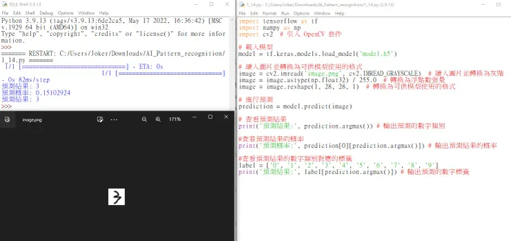
測試

import tensorflow as tf
import numpy as np
import cv2  # 引入 OpenCV 套件
# 載入模型
model = tf.keras.models.load_model('model.h5')
# 讀入圖片並轉換為可供模型使用的格式
image = cv2.imread('image.png', cv2.IMREAD_GRAYSCALE)  # 讀入圖片並轉換為灰階
image = image.astype(np.float32) / 255.0  # 轉換為浮點數張量
image = image.reshape(1, 28, 28, 1)  # 轉換為可供模型使用的格式
# 進行預測
prediction = model.predict(image)
# 查看預測結果
print('預測結果:', prediction.argmax()) # 輸出預測的數字類別
#查看預測結果的概率
print('預測概率:', prediction[0][prediction.argmax()]) # 輸出預測結果的概率
#查看預測結果的數字類別對應的標籤
label = ['0', '1', '2', '3', '4', '5', '6', '7', '8', '9']
print('預測結果:', label[prediction.argmax()]) # 輸出預測的數字標籤