《從零開始的資料科學筆記》Day#15: 房價如何預測?

在學習完機器學習的各種基礎知識後，我們終於可以開始進入實際應用的階段。機器學習的常見應用大致可分為四大類：迴歸（Regression）、分類（Classification）、分群（Clustering）、以及時間序列分析（Time Series Analysis）。身為資料科學家，理解並掌握這些方法的原理、適用情境以及實作技巧，才能在面對不同商業與研究問題時選擇正確的解決方案。

我們將從 迴歸分析 開始探索。

📌 什麼是迴歸分析？

迴歸分析是一種用來預測連續數值的統計與機器學習方法。它透過分析「輸入特徵（features）」與「目標變數（target）」之間的關係，建立一個數學模型，並用這個模型來預測新的資料點可能的結果。

🎯 常見應用情境

• 根據房屋特徵（坪數、地段、房齡）預測房價
• 根據行銷花費預測銷售額
• 根據病患檢查數據預測血糖值或血壓
• 根據天氣條件預測氣溫或電力需求

🧾 0. 環境建議與可重現性

通常資料科學家會使用虛擬環境或是容器來建立開發環境，由於比較複雜所以會在後續的筆記中說明，這邊先直接在本機端開發即可。

使用Ipython notebook相關的IDE開發:

pip install numpy pandas scikit-learn matplotlib seaborn joblib

設定亂數種子，使每次實驗的資料子集可以保持一致：

RANDOM_STATE = 42

📦 1. 資料集說明（Dataset Card）

• 名稱：California Housing Dataset
• 來源：sklearn.datasets.fetch_california_housing()
• 任務：迴歸（預測房價中位數）
• 樣本數：20640
• 特徵數：8 個連續特徵
• 目標變數：MedHouseVal（單位：以十萬美元為單位）

🔎 2. 載入與初探（Loading & Quick EDA）

• 透過統計分析與視覺化圖表，初步了解並掌握資料的狀況
• 決定後續的資料前處理如何進行
• 如:缺失值理處、異常值處理和資料轉換等步驟

import numpy as np
import pandas as pd
import matplotlib.pyplot as plt
import seaborn as sns
from sklearn.datasets import fetch_california_housing

data = fetch_california_housing()
X = pd.DataFrame(data.data, columns=data.feature_names)
y = pd.Series(data.target, name="MedHouseVal")

print(X.shape)
print(X.head(3))
print(y.describe())
print("Missing:", X.isna().sum().sum())

sns.histplot(y, bins=50)
plt.title("Target Distribution (Median House Value)")
plt.show()

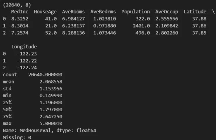
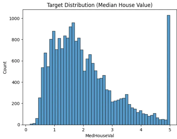
從分析結果可以知道:

• 沒有缺失值
• Y欄位在數值等於5的數量特別多，這是因為當初資料收集時有設定上限，導致超過5以上的值都設為5

🧼 3. 資料前處理（Preprocessing）

• 由於沒有缺失值，不需要做額外處理
• 將X跟Y依比例切分成train和test子集
• 設定標準化處理，後續使用

from sklearn.model_selection import train_test_split
from sklearn.preprocessing import StandardScaler

X_train, X_test, y_train, y_test = train_test_split(
    X, y, test_size=0.2, random_state=RANDOM_STATE
)
print(f'X_train.shape: {X_train.shape}')
print(f'y_train.shape: {y_train.shape}')
print(f'X_test.shape: {X_test.shape}')
print(f'y_test.shape: {y_test.shape}')

scaler = StandardScaler()

X_train.shape: (16512, 8)
y_train.shape: (16512,)
X_test.shape: (4128, 8)
y_test.shape: (4128,)

🧩 4. 特徵工程（Feature Engineering）

• 可加入衍伸特徵，例如：房間數/家庭數、臥室比例、人口密度。
• 或是進行特徵篩選，選出重要性較高的特徵
• 類別型的特徵也需要在這將其轉換為數值型
• 亦可進一步引入Box-cox轉換來修正特徵的資料分布

X_train = X_train.copy()
X_test = X_test.copy()
X_train["rooms_per_household"] = X_train["AveRooms"] / X_train["HouseAge"]
X_test["rooms_per_household"] = X_test["AveRooms"] / X_test["HouseAge"]

🧪 5. 基準模型（Baseline）

進行模型訓練實驗時，需要先設定一個基準模型，將其當作每次實驗的比較基準，通常會使用較簡單的模型。

from sklearn.dummy import DummyRegressor
from sklearn.metrics import root_mean_squared_error

baseline = DummyRegressor(strategy="mean")
baseline.fit(X_train, y_train)
y_base = baseline.predict(X_test)
print("Baseline RMSE:", root_mean_squared_error(y_test, y_base))

Baseline RMSE: 1.1448563543099792

🧠 6. 模型選擇與 GridSearchCV

選擇不同的模型和參數的設置進行模型選擇實驗，自動讓他搜尋最佳模型與參數，然後印出各種相關資訊。

from sklearn.linear_model import LinearRegression, Ridge
from sklearn.ensemble import RandomForestRegressor
from sklearn.pipeline import Pipeline
from sklearn.model_selection import GridSearchCV, KFold
from sklearn.preprocessing import StandardScaler
import pandas as pd
import numpy as np

# 假設 RANDOM_STATE 已經定義，如果沒有則設定一個
RANDOM_STATE = 42

pipe = Pipeline([
    ("scale", StandardScaler()),
    ("model", LinearRegression())
])

param_grid = [
    {"model": [LinearRegression()]},
    {"model": [Ridge()], "model__alpha": [0.1, 1.0, 10.0]},
    {"model": [RandomForestRegressor(random_state=RANDOM_STATE)],
     "model__n_estimators": [100, 300], "model__max_depth": [None, 10, 20]}
]

cv = KFold(5, shuffle=True, random_state=RANDOM_STATE)
grid = GridSearchCV(pipe, param_grid, scoring="neg_root_mean_squared_error", cv=cv, n_jobs=-1)
grid.fit(X_train, y_train)
print("Best CV RMSE:", -grid.best_score_)

# 新增以下部分：列出最佳模型與參數
print("\n" + "="*50)
print("最佳模型詳細資訊")
print("="*50)

# 獲取最佳模型名稱
best_model_name = grid.best_estimator_.named_steps['model'].__class__.__name__
print(f"最佳模型: {best_model_name}")

# 獲取最佳模型參數
best_params = grid.best_params_
print("\n最佳參數:")
for param, value in best_params.items():
    if param != "model":  # 跳過模型本身的參數
        print(f"  {param}: {value}")

# 如果想更詳細地了解模型的參數，可以顯示所有參數
print("\n最佳模型的所有參數:")
best_model = grid.best_estimator_.named_steps['model']
model_params = best_model.get_params()
for param, value in model_params.items():
    print(f"  {param}: {value}")

# 顯示交叉驗證的詳細結果
print("\n" + "="*50)
print("交叉驗證結果詳細資訊")
print("="*50)

# 將CV結果轉換為DataFrame以便查看
cv_results = pd.DataFrame(grid.cv_results_)

# 選擇需要顯示的列
columns_to_display = ['mean_test_score', 'std_test_score', 'rank_test_score', 'params']
cv_results_display = cv_results[columns_to_display]

# 將結果按rank_test_score排序
cv_results_sorted = cv_results_display.sort_values('rank_test_score')

# 轉換negative RMSE為positive RMSE以便理解
cv_results_sorted['mean_test_score'] = -cv_results_sorted['mean_test_score']
cv_results_sorted['std_test_score'] = cv_results_sorted['std_test_score']

# 重命名列以便理解
cv_results_sorted = cv_results_sorted.rename(columns={
    'mean_test_score': 'RMSE (mean)',
    'std_test_score': 'RMSE (std)',
    'rank_test_score': 'Rank'
})

# 顯示前5名模型
print("Top 5 models based on cross-validation:")
pd.set_option('display.max_colwidth', None)  # 確保params列顯示完全
print(cv_results_sorted.head(5))

# 顯示最佳模型的測試分數
print("\n" + "="*50)
print("最佳模型在測試集上的表現")
print("="*50)
test_score = -grid.score(X_test, y_test)  # 因為是neg_root_mean_squared_error，所以取負值
print(f"Test RMSE: {test_score:.4f}")

# 獲取特徵重要性（如果模型支持）
if hasattr(best_model, 'feature_importances_'):
    print("\n" + "="*50)
    print("特徵重要性")
    print("="*50)
    # 假設X_train是DataFrame且有列名
    if hasattr(X_train, 'columns'):
        feature_names = X_train.columns
    else:
        feature_names = [f"Feature {i}" for i in range(X_train.shape[1])]
    
    importance = best_model.feature_importances_
    features_importance = pd.DataFrame({
        'Feature': feature_names,
        'Importance': importance
    }).sort_values('Importance', ascending=False)
    
    print(features_importance)

Best CV RMSE: 0.5133453106680681

==================================================
最佳模型詳細資訊
==================================================
最佳模型: RandomForestRegressor

最佳參數:
  model__max_depth: None
  model__n_estimators: 300

最佳模型的所有參數:
  bootstrap: True
  ccp_alpha: 0.0
  criterion: squared_error
  max_depth: None
  max_features: 1.0
  max_leaf_nodes: None
  max_samples: None
  min_impurity_decrease: 0.0
  min_samples_leaf: 1
  min_samples_split: 2
  min_weight_fraction_leaf: 0.0
  monotonic_cst: None
  n_estimators: 300
  n_jobs: None
  oob_score: False
  random_state: 42
  verbose: 0
  warm_start: False

==================================================
交叉驗證結果詳細資訊
==================================================
Top 5 models based on cross-validation:
   RMSE (mean)  RMSE (std)  Rank  \
5     0.513345    0.013247     1   
9     0.513383    0.013322     2   
4     0.515307    0.012697     3   
8     0.515626    0.012716     4   
7     0.542397    0.013469     5   

                                                                                                    params  
5  {'model': RandomForestRegressor(random_state=42), 'model__max_depth': None, 'model__n_estimators': 300}  
9    {'model': RandomForestRegressor(random_state=42), 'model__max_depth': 20, 'model__n_estimators': 300}  
4  {'model': RandomForestRegressor(random_state=42), 'model__max_depth': None, 'model__n_estimators': 100}  
8    {'model': RandomForestRegressor(random_state=42), 'model__max_depth': 20, 'model__n_estimators': 100}  
7    {'model': RandomForestRegressor(random_state=42), 'model__max_depth': 10, 'model__n_estimators': 300}  

==================================================
最佳模型在測試集上的表現
==================================================
Test RMSE: 0.5102

==================================================
特徵重要性
==================================================
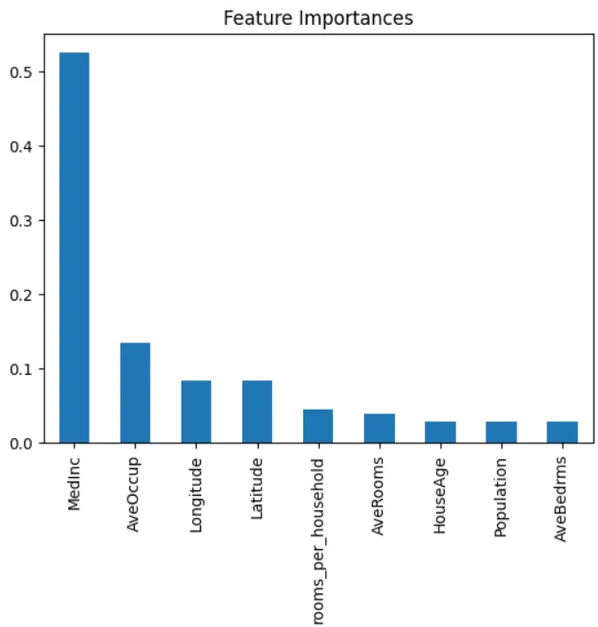
               Feature  Importance
0               MedInc    0.524881
5             AveOccup    0.135404
7            Longitude    0.084010
6             Latitude    0.083968
8  rooms_per_household    0.044613
2             AveRooms    0.040032
1             HouseAge    0.029529
4           Population    0.029080
3            AveBedrms    0.028483

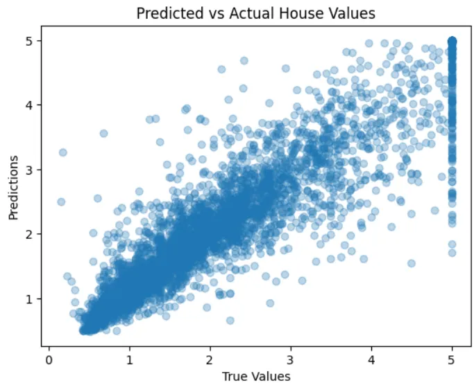
📏 7. 模型評估

• 使用最佳模型來進行模型評估，通常會同時考慮多個評估指標，以多種角度來評估此模型。
• AIC和BIC也是常用的模型選擇方式

from sklearn.metrics import mean_absolute_error, root_mean_squared_error, r2_score

best_model = grid.best_estimator_
y_pred = best_model.predict(X_test)

print("MAE:", mean_absolute_error(y_test, y_pred))
print("RMSE:", root_mean_squared_error(y_test, y_pred))
print("R²:", r2_score(y_test, y_pred))

plt.scatter(y_test, y_pred, alpha=0.3)
plt.xlabel("True Values")
plt.ylabel("Predictions")
plt.title("Predicted vs Actual House Values")
plt.show()

MAE: 0.3305970771075585
RMSE: 0.5102476192195154
R²: 0.8013195595861359

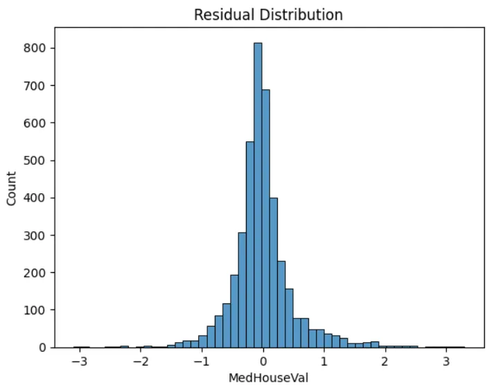
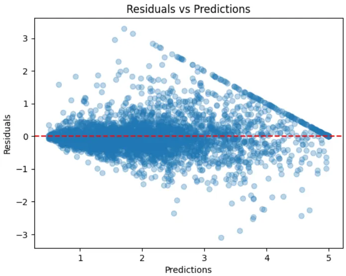
🔍 8. 殘差分析（Residual Analysis）

殘差分析主要檢查兩件事情:

• 殘差是否呈現常態分布
• 殘差是否隨機分布在零線的週圍，無明顯模式

詳細內容會在之後的筆記中說明

residuals = y_test - y_pred
sns.histplot(residuals, bins=50)
plt.title("Residual Distribution")
plt.show()

plt.scatter(y_pred, residuals, alpha=0.3)
plt.axhline(0, color="red", linestyle="--")
plt.xlabel("Predictions")
plt.ylabel("Residuals")
plt.title("Residuals vs Predictions")
plt.show()

📐 9. 特徵重要性（Feature Importance）

特徵重要性是用來篩選特徵以及判斷模型是否訓練正確的一個步驟，常使用的方式除了相關係數、統計檢定和Shapley Value之外，也有些模型內建特徵篩選功能如:Random Forest、Lasso Regression和XGBoost等。

if hasattr(best_model.named_steps['model'], 'feature_importances_'):
    importances = best_model.named_steps['model'].feature_importances_
    pd.Series(importances, index=X_train.columns).sort_values(ascending=False).plot(kind='bar')
    plt.title("Feature Importances")
    plt.show()

💾 10. 模型保存與載入

模型訓練完之後須要將其儲存起來，後續使用時再載入模型，對新資料進行預測。 要特別注意的是，模型在訓練時進行過的前處理和轉換，對新資料也要做一樣的事情，才可以讓模型預測，這部分就不特別操作了。

import joblib

joblib.dump(best_model, "california_best_model.joblib")
model = joblib.load("california_best_model.joblib")

y_pred = model.predict(X_test)