使用R語言跑多層次模型:Random intercepts model with level-2 predictor

介紹

多層次模型中的 Random intercepts model with level-2 predictor 是一種層級 2 預測變量預測層級 1 結果變量的模型。又稱為截距作為結果模型(Intercepts as outcomes model)。因為在Level 2來看其加入一個或多個層次 2 預測變項來解釋截距。

以下是 模型的一般方程式：

Level 1:​
層級 1 結果變量 = β0 +  e
Level 2:
β0 = β00 + β1 * 層級 2 預測變量 + e00

Combined:​
層級 1 結果變量 =  β00 + β1 * 層級 2 預測變量 + e00 + e​

其中：

• β00 是層級 2截距，表示當層級 2 預測變量的斜率(β1 )為0時，所有群組的層級 1 結果變量的平均值。固定效果。
• β1 是層級 2斜率係數，表示層級 2 預測變量在層級 1 結果變量中每增加一個單位時的平均變化。固定效果。
• e00 是層級 2截距的隨機效應，表示層級 2群組間截距的變異量。隨機效果。
• e 是residual，層級 1變異量。隨機效果。
• e 和e00 必須是不相關的才符合前提假設
• e 和e00 必須是常態分配才符合前提假設

如下圖，截距具有隨機效果就是認為截距會因為學校不同而有變化，所以每條線起點有差異。

範例

# 載入相關套件
library(lme4)

# 生成數據
set.seed(1234)

# 層級 1 結果變量
math_score <- rnorm(1000, mean = 50, sd = 10)

# 層級 2 預測變量
school_ses <- rnorm(50, mean = 50, sd = 10)

# 合併數據，並命名為df
df <- data.frame(math_score, school_ses)

# 跑模型
model <- lmer(math_score ~ school_ses + (1|school_ses), data = df)

# 檢視模型結果
summary(model)

以下是這個模型的 R 語言程式碼的詳細解釋：

• library(lme4)：載入 lme4 套件，該套件用於擬合多層次模型。
• set.seed(1234)：設定隨機種子，以便每次生成數據時得到相同的結果。
• math_score <- rnorm(1000, mean = 50, sd = 10)：生成 1000 個學生級數學成就數據，平均值為 50，標準差為 10。
• school_ses <- rnorm(50, mean = 50, sd = 10)：生成 50 個學校級 SES 數據，平均值為 50，標準差為 10。
• df <- data.frame(math_score, school_ses)：合併層級 1 和層級 2 數據。
• model <- lmer(math_score ~ school_ses + (1|school_ses), data = df)：擬合Random intercepts model with level-2 predictor 模型。
• summary(model)：檢視模型結果。

範例中我們合併數據，並命名為df，df 資料是隨機生成的數據，包含 1000 個觀察值的數據庫，其中包含兩個變量：

• math_score：學生數學成就(層級 1 結果變量)是連續變量，其值範圍為 0 到 100。
• school_ses：學校社會經濟地位SES(層次2預測變項)也是連續變量，其值範圍為 0 到 100。層級 2 預測變量代表，同個學校內具有一樣的社會經濟地位。
• 同時呢，我們也把school_ses當作學校ID，因為它只有50個不同的數字，也可以代表50間不同的學校ID。

可以使用 head() 函數來查看 df 資料的前幾個觀察：

math_score school_ses
1 47.2676 48.5566
2 52.7324 51.4434
3 54.2072 52.3302
4 49.2428 49.5266
5 51.7176 50.4134
...

接下來model <- lmer(math_score ~ school_ses + (1|school_ses), data = df) 跑模型​的結果如下：

Linear mixed model fit by REML. t-tests use Satterthwaite's method [
lmerModLmerTest]
Formula: math_score ~ school_ses + (1 | school_ses)
   Data: df

REML criterion at convergence: 7441.3

Scaled residuals: 
    Min      1Q  Median      3Q     Max 
-3.3469 -0.6451 -0.0023  0.6410  3.2528 

Random effects:
 Groups     Name        Variance Std.Dev.
 school_ses (Intercept)  0.00    0.000   
 Residual               99.48    9.974   
Number of obs: 1000, groups:  school_ses, 50

Fixed effects:
             Estimate Std. Error        df t value Pr(>|t|)    
(Intercept)  48.27024    1.56857 998.00000  30.774   <2e-16 ***
school_ses    0.03043    0.03194 998.00000   0.953    0.341    
---

從模型結果中可以看到，層級 2 預測變量 school_ses 的斜率係數為 0.030，顯著性水平未達顯著。這表明，學校級 SES 與學生級數學成就之間沒有顯著關聯。另外我們發現school_ses (Intercept)為0.00，代表<.01的意思，可見學校的Random effects非常小，幾乎沒有忽略，這也難怪，畢竟這是隨機生成的資料。

若不想使用REML估計法可以改用ML估計法: lmer(前面一樣..., REML = F)

最重要的是，我們能從上面數據代入Random intercepts model with level-2 predictor 模型公式:

Level 1:​
math_score = β0 +  99.48
Level 2:
β0 = 48.27024 + 0.03043 * school_ses + (<.01)

Combined:​
math_score =  48.27024 + 0.03043 * school_ses + (<.01) + 99.48

接下來畫一張圖來看

# 載入相關套件 
 library(ggplot2)
# 繪製圖形
ggplot(df, aes(school_ses, math_score)) +
  geom_point() +
  geom_line(aes(school_ses, fitted(model))) +
  labs(x = "School SES", y = "Math scores")

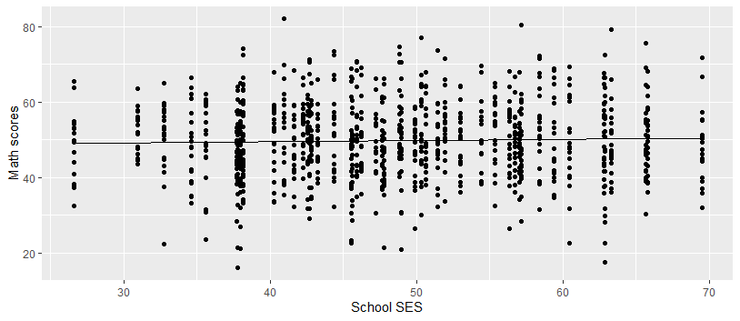
跑出來就是下圖，X軸表示學校級 SES，Y軸表示學生級數學成就。黑色線是模型的預測線，果然兩者關聯很小。每個學生都是一個黑點，可以看出來同樣的學校級 SES，但在數學成就相差很大，所以呈現[I]分散形狀。

您的研究遇到了統計分析的困難嗎？您需要專業的統計諮詢和代跑服務嗎？請點我看提供的服務